By RAFAŁ WAŚKO (Predictive Solutions)
The main idea of regression is to predict the value of a dependent variable (otherwise known as predictor, explained variable) based on one or more independent variables (called predictors, explanatory variables).
The simplest form of regression is simple linear regression, which assumes using only one predictor to explain the dependent variable. It is worth noting, however, that there are many more regression techniques that allow the construction of very complex models that can be used in business, but also in other areas such as manufacturing, weather forecasting, trade, health care, or agriculture. As an example, we can indicate the prediction of car value, based on the engine capacity, its mileage and the number of years of its use. Another example might be a linear regression model in which we want to predict the amount of income based on such predictors as the number of years of schooling, level of intelligence, social capital, or parental education. Of course, the number of practical applications is much, much larger. We are limited only by our imagination and the need to stick to several assumptions (I will explain them below).
WHAT IS REGRESSION ANALYSIS?
The analyst prepares a so-called regression model to answer the question of what value a variable will take when we know the value of another variable. Using a more scientific definition, regression can be defined as a statistical technique that allows us to describe the co-variance of several variables by fitting functions to them. In regression analysis we can distinguish two main objectives: to examine the size and structure of the relationship between variables (1) and to predict the value of one variable based on the relationship with another variable or set of variables (2).
EQUATION OF SIMPLE LINEAR REGRESSION
The equation for a simple linear regression is similar to the equation of a linear function. We can write the formula for linear regression:
Where:
y – dependent variable (explained variable, predictor),
x – independent variable (predictor),
a – free expression, otherwise referred to as a constant,
x – regression coefficient, otherwise known as the directional coefficient.
To calculate the regression coefficient use the formula:
Where:
b – regression coefficient,
xi – results for the independent variable, consecutive observations of the explanatory variable,
yi – results for the dependent variable, consecutive observations of the explanatory variable,
x – mean value of the independent variable,
y – mean value of the dependent variable.
The calculation of the free expression is already simple. For this, we use the regression coefficient calculated earlier and the average value for the independent variable and the dependent variable.
INTERPRETATION OF REGRESSION COEFFICIENT AND FREE EXPRESSION
In simple linear regression, two main coefficients are determined. The first is the coefficient b, or the unstandardized regression coefficient. Referring to the regression line, this measure determines the angle of slope of the line with respect to the X axis. It is also otherwise known as the directional coefficient. By substituting the values into the linear regression formula, the regression coefficient determines how much the value of the dependent variable will increase or decrease if the predictor value changes by one unit. The coefficient b in a linear regression model is necessary to predict the value of the dependent variable. To obtain linear regression coefficients we can use the least squares method (MNK). This method involves minimizing the sum of the squares of the distances of all points from the desired straight line.
In the case of free expression, this measure provides us with information on what value the dependent variable can take if the predictor is zero. It is worth noting, however, that in this case the results should be interpreted with caution. The value of free expression can be negative, but it does not mean that the independent variable can also take on negative values, e.g. in the model in which we predict the number of calories in beer (dependent variable) on the basis of alcohol content (independent variable), the value of free expression can be negative, which does not mean that non-alcoholic beer will have negative calories.
LINEAR REGRESSION ASSUMPTIONS
Linear regression allows the use of quantitative variables with normal distributions. However, before conducting a regression analysis, the analyst should make sure that the assumptions for this statistical technique are met.
Four major assumptions associated with the linear regression model can be identified:
• Linearity – there is a linear relationship between the independent variable and the dependent variable.
• Homoskedasticity – the variance of the residuals is the same for all observations.
• The random component (residuals) are uncorrelated and have a normal distribution.
• Independence of variables – none of the independent variables can be correlated with another independent variable (applies to multivariate regression).
EXAMPLE OF SIMPLE LINEAR REGRESSION
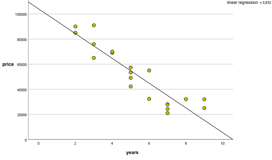
Let’s look at a simple example where we want to predict car prices (the dependent variable) based on the number of years a car has been in existence (the independent variable, the predictor). Of course, the price of a car can be influenced by other variables as well, but for the purpose of introducing the reader to linear regression, I will use only one predictor. In linear regression analysis, as the name suggests, we assume that the relationship between two variables is a linear relationship. Representing the data on a scatter plot, we see that the variables are negatively correlated, i.e. as the years of a car increase, its price decreases[1].
Figure 1. Relationship of used car price to number of years with the regression line
In linear regression analysis, we want to draw a line that best fits the points we see on the scatter plot. We can use the method of least squares, which allows us to draw a regression line that best fits the collected data. To do that, we calculate the coefficient b (regression coefficient) and the value of free expression a.
After calculating these values, we can insert them into the formula for simple linear regression. For our data, the parameters are:
• regression coefficient (b) = -9860,
• free expression (a) = 104 029.
We can therefore write the linear regression equation as follows:
Price = 104029 – 9860 * years
By interpreting the regression coefficient, we can say that with each passing year, the car will lose 9860 PLN in value. In the case of a free expression, the value of PLN 104,029 represents the amount that would have to be paid for a new car.
If the analyst wants to predict the price of the next car, it is enough to add to the formula the number of years of the car for which we want to make a prediction. For example, for a car that is 6 years old, the result would be PLN 44,869.


