By (Predictive Solutions)
This procedure is intended to make life easier for those who work on large datasets and want to use regression models. Automatic linear models lack many advanced settings and options for model exploration that can be found in other regression procedures. On the other hand, as with other procedures of this kind, it speeds up and streamlines data processing.
What are the differences?
Regression analysis in PS IMAGO PRO traditionally employs the Linear Regression procedure found in SPSS Statistics (REGRESSI0N). However, in version 19 and higher SPSS Statistics has an additional procedure, namely LINEAR. This procedure is used widely in predictive analyses and will be the focus of this and subsequent blog posts.. Both regression methods have pros and cons, advocates and opponents. Today, we will focus on the potential benefits of using the LINEAR procedure and how to build a simple model and use its results.
The traditional regression procedure offers numerous techniques for choosing variables for the model. These techniques belong to the family of progressive methods (such as stepwise, forward selection, or backward elimination). The variables are selected automatically using statistical criteria, namely a sequence of t or F tests. The LINEAR procedure additionally provides a method referred to as all possible subsets.
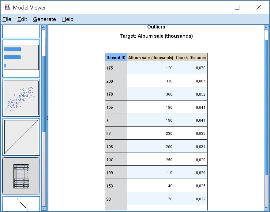
The regression model (REGRESSION) enables the analyst to carry out an in-depth analysis of outliers and influencing observations. Statistics such as Cook’s distance or DFBETAS can be saved to the dataset, something which is not possible when a model is generated automatically using the LINEAR function. Instead, such observations are handled when the model is being built, i.e., the application automatically decides which observation should be considered an outlier.
The third feature of the LINEAR procedure is the option to build so-called ensemble models, for example, through bagging or boosting.
Its fourth advantage is the ability to adapt it to process large datasets. This, however, requires PS IMAGO PRO in a client/server setup.
What’s in the box?
First, we will have a look at the interface of the Automatic linear modeling window and its result objects. We will also look at options for automatic preparation of data available for the procedure. Then, we will focus on the methods for selecting predictors and on building ensemble models.
By way of illustration, we will build a sample regression model to verify whether or not there is a linear relationship between the sales of music CDs and such features as:
- audience artist score
- advertising spending
- number of radio plays
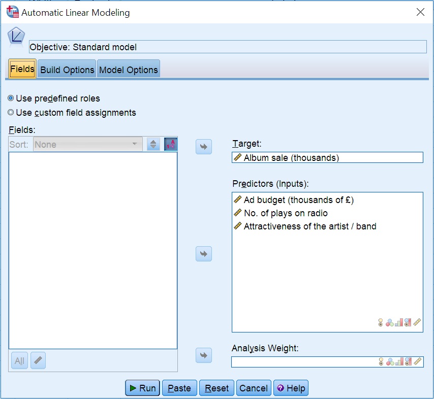
The procedure can be found in menu Analyze > Regression > Automatic Linear Modeling. Go to the Fields tab and select variables for the analysis.
Another similarity is the possibility to declare a role for a variable (Data Editor > Variable View > Role). If you declare a role as Input or Target, Automatic linear modeling will automatically place the variables into the relevant fields.
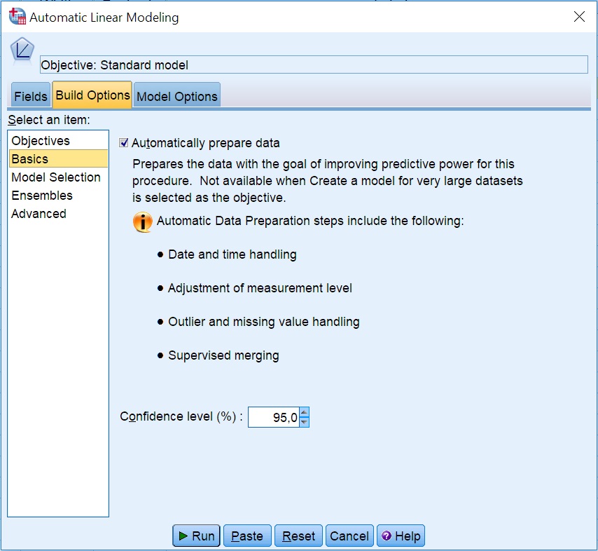
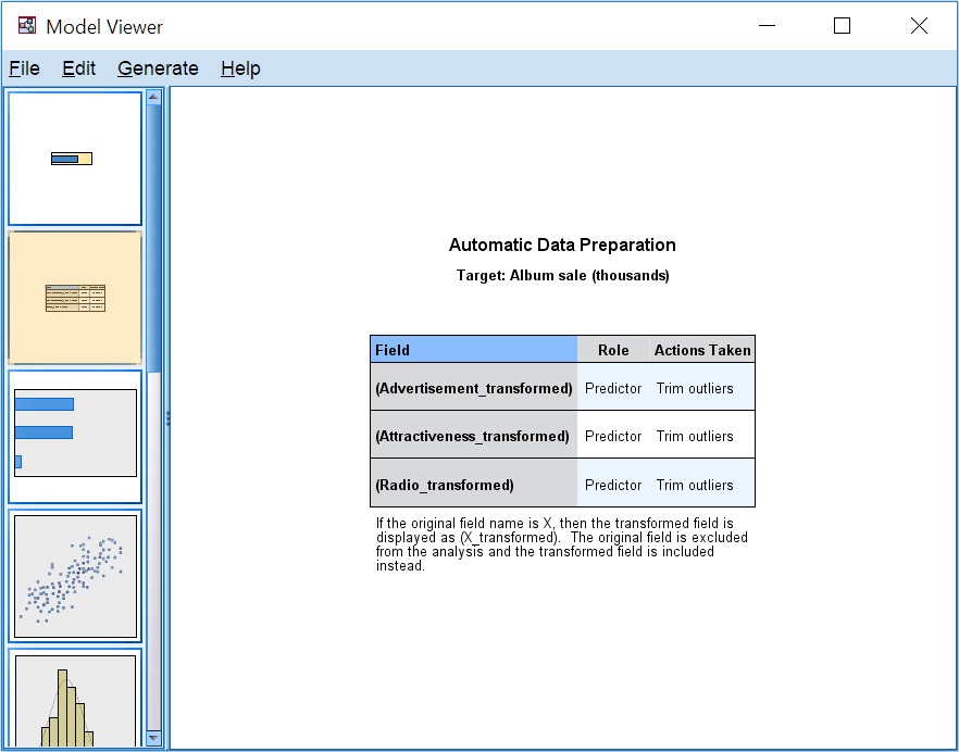
Go to the Build Options tab. The list on the left-hand side shows a number of option groups. Today, we will focus on Basics which is where you can enable automatic data preparation, as shown in Fig. 2. Most of the transformations improve the predictive power of the model. If you enable this option, the model will be built from processed values, not the original variables. The transformations used are saved with the model. The transformations implemented when this option is enabled are:
- Date and time handling – date and time predictors will be converted into a duration, a number, for example, of months from today.
- Adjustment of measurement level – variables declared to be quantitative variables with less than five unique values will be treated as ordinal variables. Ordinal variables with more than ten categories will be treated as quantitative variables.
- Outlier handling – values not within +/- three standard deviations from the mean are considered outliers.
- Missing value handling – missing values of qualitative variables are replaced with a modal for a nominal scale and a median for an ordinal scale. Missing values in quantitative variables are replaced with a mean value.
- Supervised merging – before qualitative variables are handled in the model, the system verifies whether or not it is important for predicting the target variable to retain information on all categories in a variable. If the predictor is a qualitative variable, (such as education), you can check whether the identified categories are correct. Do the categories of education differentiate earnings well? Too many detailed categories can make it more difficult to identify general dependencies. In the case of regression models, qualitative variables are converted into a set of boolean variables before they are used. By using variables with fewer categories, you simplify and generalise the model. Variables whose categories do not differentiate the predicted variable are not used in the model.
You can additionally set the confidence interval at which the interval estimation of the model’s parameters will be carried out. It is usually from 0.9 to 0.99.
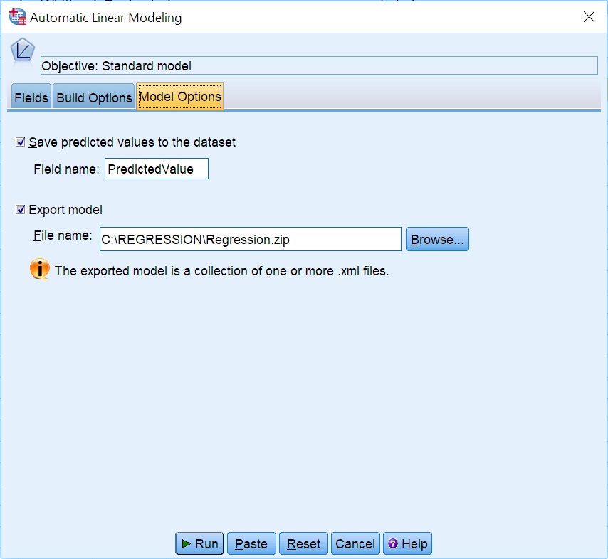
Go to the Model Options tab. Here, you can make decisions regarding the saving of the model. If you want the predicted sales volume to be included in the dataset, you need to enable the first option, which is disabled by default: Save predicted values to the dataset, and select the name for the predicted value variable.
The model summary
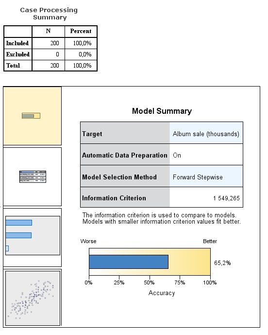
The summary shows general information about the model and adjusted R2 as a percentage bar chart. We get 65.2%, which may be satisfactory depending on the field.
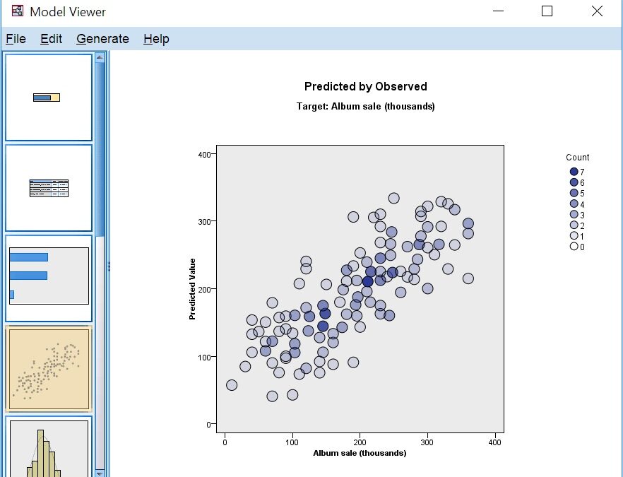
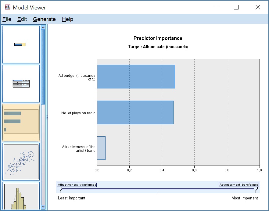
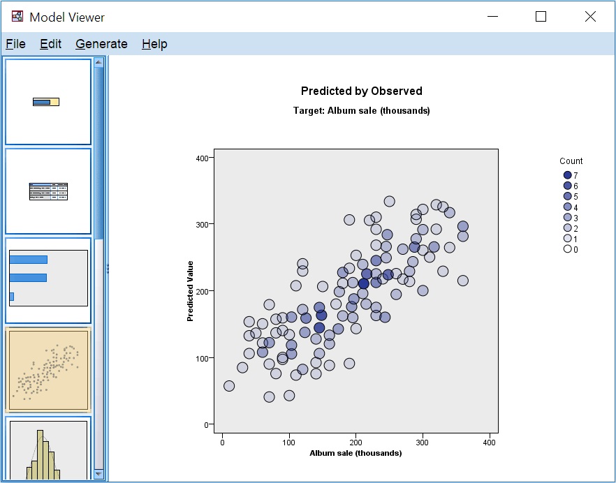
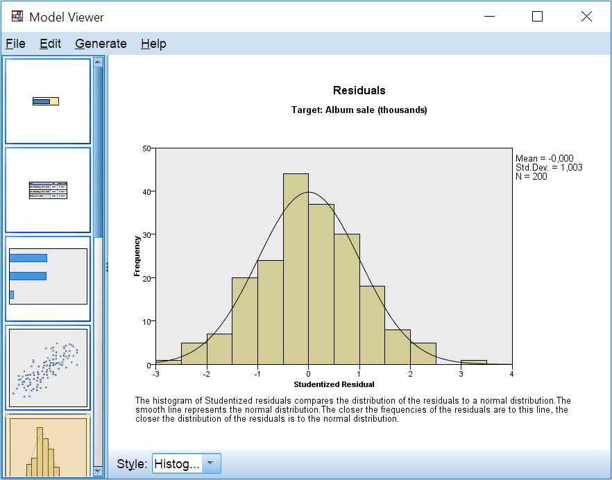
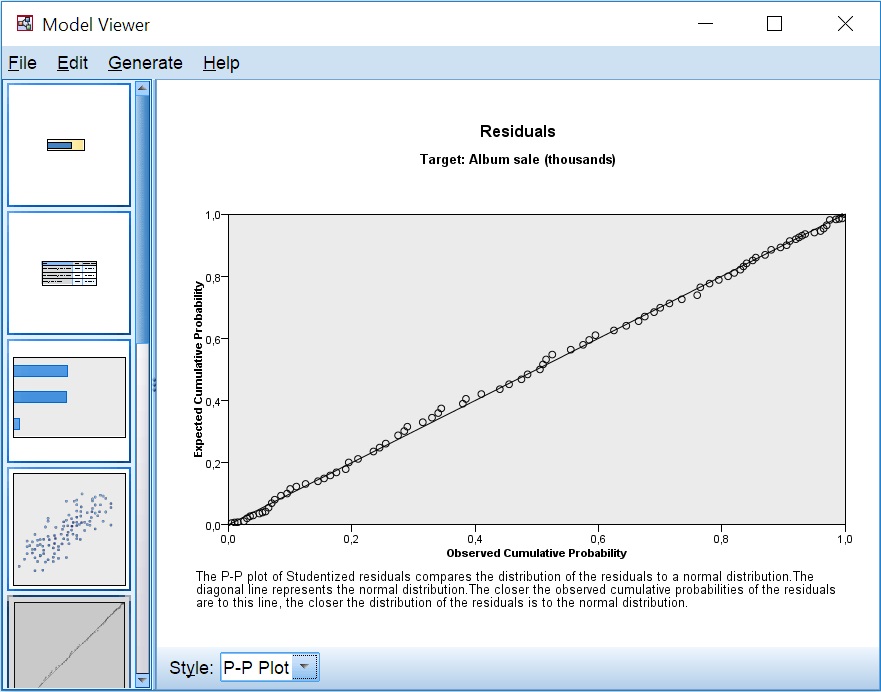
By double-clicking on the report, you open a model viewer window where you can see other results. You navigate the report by clicking on the objects on the left-hand side. The first object we have seen already, solet’s see what is further down.
Although automatic procedures are controversial, they can be useful. This approach is usually justifiable for large datasets where automatic procedures facilitate using the computing power for searching and preliminary exploration of data. In future posts, we will look more into model building and the options you can change when building models using Automatic linear modeling.

